Final Report

Project Overview

This E155 final project sought to create a karaoke machine. The design allows users to choose a song to sing, displaying lyrics and playing the song as a guide via speaker, and ultimately compares the user’s singing to the expected frequencies, displaying both a letter grade and a percent error (between received and expected frequencies) after a song finishes. The main input is a MEMS digital microphone, which goes through digital signal processing and FFT to pick up the correct frequencies at which people speak into the microphone. The LCD screen functions as the principal user interface, directing users to choose songs, displaying lyrics, and presenting grades.

Project Specifications

Design allows the user to choose a song through external hardware
Design detects input frequencies between 300 to 2000 Hz
Design scores the user’s singing by comparing detected and expected notes
Design plays back the expected song through a speaker as reference
Design utilizes a pitch and delay media format (as seen in Lab 4)
Displays properly-timed lyrics on an LCD screen
LCD display does not flicker

Bill of Materials

Part Name	Part Number	Quantity	Price	Vendor
Adafruit PDM MEMS Microphone Breakout	MP34DT01-M	1	$11.23 ($4.95 part, $6.28 shipping + tax)	Adafruit
Hosyond I2C 2004 LCD Module	HD44780U	1	$26.32 ($16.99 part, $6.99 shipping, $2.34 estimated tax)	Amazon
TOTAL			$37.55

Table 1: Bill of materials

Design Details

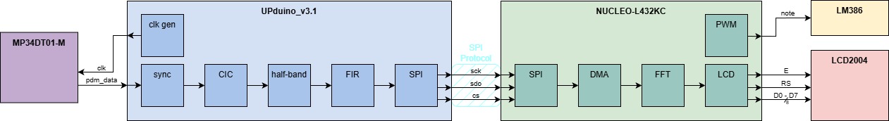
The general, high-level overview of our project — with all of the protocols used explicitly outlined — can be viewed in Figure 1 below:

New Non-Trivial Hardware

The two new, non-trivial pieces of hardware that are used in this project are the Adafruit PDM microphone and the Hoysond LCD module.

Adafruit PDM Microphone

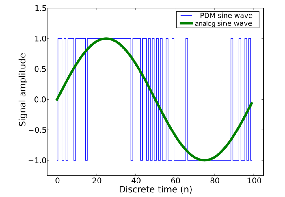
We used a MP34DT01-M, a MEMS digital microphone. It outputs data in Pulse-Density Modulation (PDM) format, which is a format of representing an analog signal in a single bit, with the density of 1’s and 0’s reflecting the amplitude of the signal.

This microphone itself took 4 inputs: a 3.3V power supply, a ground, a L/R channel selector for simplified stereo applications, and a synchronization input clock. The input clock was valid between frequencies of 3.25 to 1 MHz, which meant we were able to select a frequency and drive it from the FPGA. We chose to ground L/R out of default. The output was the Dout pin, and could be read by an FPGA pin in PDM format. The clock and Dout were connected directly to the FPGA board to minimize lag and voltage drop.

Within E155, there has been no usage of this PDM format. The closest data format or acquisition method we had gone over was quadrature encoders, which we used in Lab 5. They were able to represent analog motion in two 1-bit digital signals, but PDM is a distinct method of representing analog waves in a single bit, which is beyond the previous material of this course.

Hoysond LCD Module

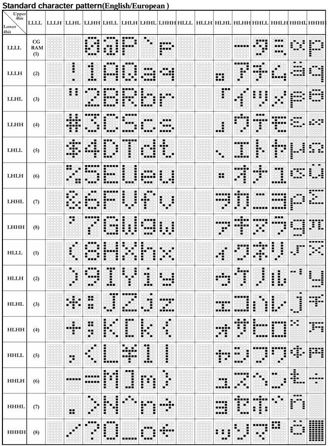
The LCD used seems to comprise the HD44780 Hitachi controller chip, as well as a PCF8574A bit-expander for I2C interfacing. The screen itself has four rows and 20 columns — or, in other words, 80 total spaces — with which to write characters of its user’s choosing. It needs 5 V of power to display characters properly, with the ability to adjust both its backlight brightness and contrast. There are two options for sending it instructions: either over I2C or directly through its 11-pin parallel interface, including:

1 Enable bit (E)
1 Register Select bit (RS)
1 Read/Write bit (RW)
8 data pins (D0 - D7)

More specifics about these pins and their respective functionalities can be found in the datasheet for the LCD’s Hitachi controller, specifically. Regardless, for both methods of communication, the module uses the sequences of high and low voltages detected in tandem with a look-up table, with each operation having its own lead-in op-code (such as the Set Address and Clear Display functions) and each character having its own unique sequence associated with it. The latter can be viewed rather clearly in Figure 2, as follows:

Note that if you decide to communicate with the LCD by sending bits to all of its pins in parallel, each transaction will have to be ended with a short pulse of the Enable (E) bit, so as to tell the module that its information has been completely updated.

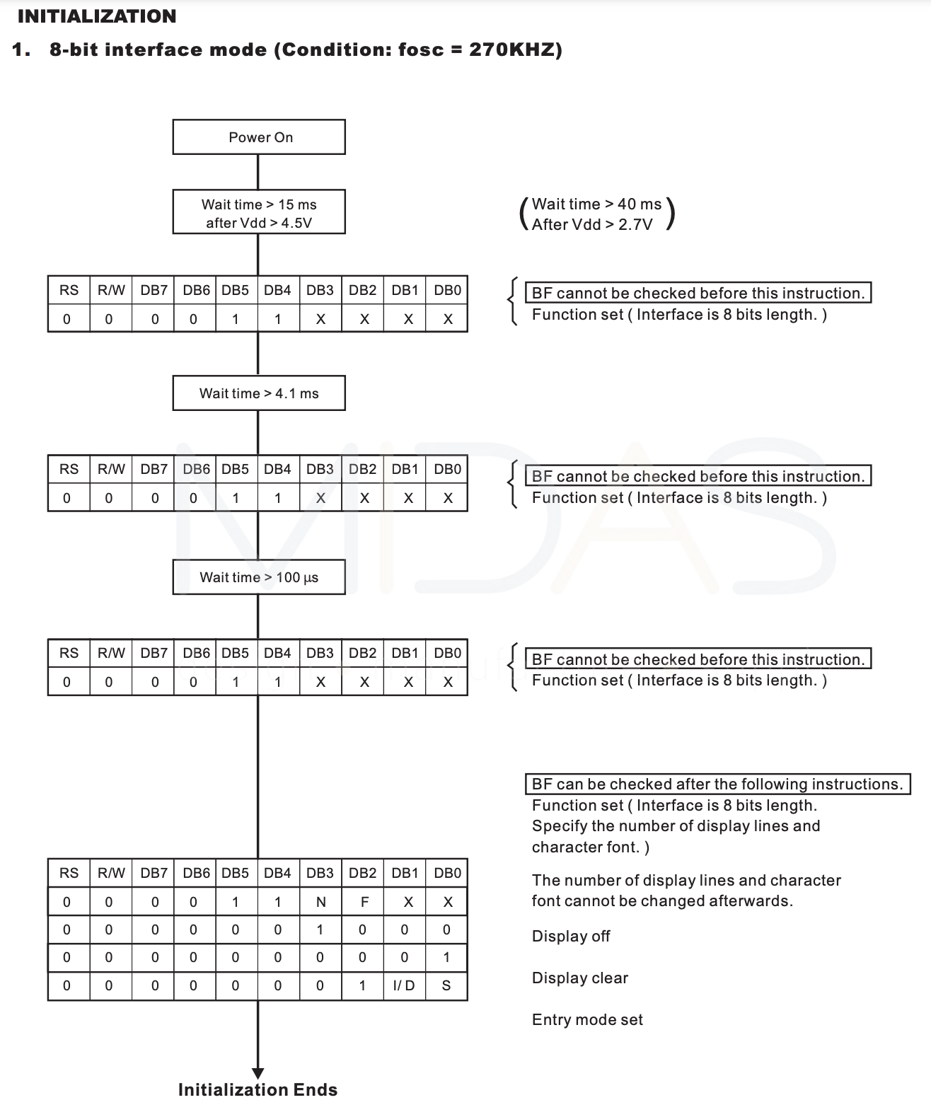
Moreover, the LCD requires a specifically-timed initialization sequence in order to fully function. This is outlined in Figure 3.

Ultimately, the features implemented with this hardware go above and beyond the previous material covered in class, as they require the configuration of an external display. More specifically, we had to learn about the different communication protocols that an LCD can use, and compare the pros and cons of both. Eventually, we came to the conclusion that using a parallel interface would be best because 1) when there are pins to spare for it, it’s the fastest, and 2) the datasheet for the PCF8574A bit-expander is vague and thus, it is extremely hard to parse how to interact with it when using I2C; in the interest of not getting hung-up over something that could be easily avoided, we decided to bypass it entirely. (See the Schematic section below for more details on some bugs that we needed to address when doing this.)

FPGA Design Overview

The FPGA is in control of the microphone, processing its data, and sending that data to the MCU. Our microphone is a MP34DT01-M, a MEMS digital microphone. We drive this using a 1.536 MHz clock signal generated by the FPGA, and the microphone outputs data in Pulse-Density Modulation (PDM) format, which is then fed back into the FPGA. PDM is a format of representing an analog signal in a single bit, with the density of 1’s and 0’s reflecting the amplitude of the Figure 4 signal.

The top module is karaoke_top.sv, as found in the GitHub’s fpga/src. The FPGA feeds the PDM signal through a pipeline of 3 digital audio filters: a CIC filter / cic.sv, half-band filter / hb.sv, and FIR filter / fir.sv.

These three filters were used to create a decimation ratio of 96, downsampling the 1.536 MHz PDM output down to a 16 kHz output. The CIC takes the brunt of the decimation with a 24 decimation ratio in 4 stages, converts the PDM to a PCM, and normalizes the output values between -1 to 1. The half-band and FIR filters create a passband from 0 to 4000 Hz, with a stopband at around 8000 Hz. Both filters have a decimation ratio of 2, and their coefficients were determined using matplotlib functions.

The three filters generate a 16-bit, 16 kHz PCM output, with a new sample indicated by a pulse. These signals are fed into the SPI module / spi.sv, which generates a CS, SCK, and SDO, acting as the controller/master in this case. All relevant testbenches are found in fpga/testbench and the ModelSim project is found in fpga/work. The MCU then receives these values, acting as the peripheral/slave, and accumulates them using the SPI peripheral, paired with the DMA peripheral.

Some difficulties we encountered:

Finding the correct filter pipeline design and the coefficients for the half-band and FIR
Minimizing resource usage
Figuring out new SPI configuration and implementing it
Synthesizing and flashing the executable

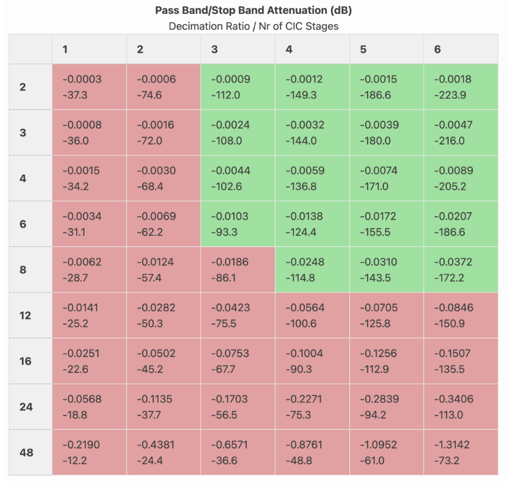
Initially, we were naively hoping to create a decimation ratio of 144, bringing a PDM input rate of 2.304 MHz down to 16 kHz. This was due to a misunderstanding of half-band filters and the resources we could fit onto the board. Half-band filters are optimized FIR filters that require only half the number of taps, and therefore multiplications, but also can only decimate (or interpolate) at a rate of 2 every filter. We had assumed that half-bands filters would be able to handle 3x and 4x decimation (which, no, is not possible) during the project proposal stage. Once we read up more on half-bands, we decided to move to a 1.536 MHz to decimate it down to 16 kHz using a decimation ratio of 96. We determined that, for our purposes, the CIC filter would be able to handle a 24 decimation ratio without much change in ripple or attenuation via this Figure 5 chart:

Since we wanted to make sure that the FIR would be able to handle everything in 16 taps to keep resource levels low, we decided to use two half-bands and keep the FIR only to minimize passband ripple and maximize stopband attenuation. However, when we loaded this onto the FPGA, there were not enough LUTs to accommodate this design. As a result, we settled on a finalized design of a 24-decimation ratio, 4-stage CIC filter, a half-band filter, and a 2x decimating and correcting final FIR filter.

When it came to determining the coefficients, we started off trying to use some MATLAB code, but switched to Python with its easier remez() function. The code for this can be found here. When it came to implementing these filters in Verilog, we mentioned that it was difficult due to resource constraints. There was some trial-and-error involved, trying to get it down from 170+% resource usage down to our final 94% LUT4 usage. Our biggest issue was the multiplications required. The FPGA only has 8 DSP blocks, and all of those were devoted to the half-band multiplications. Which meant that the CIC, FIR, and the rest of the half-band additions all had to fit their calculations in the LUTs. The CIC was generally resource-optimized already due to its perk requiring only adders and delays by design. The FIR and half-band took some tweaking. We implemented pipelining in both filters to keep the critical path short and allow the synthesis tool to map arithmetic into smaller, slower LUT-based adders rather than huge blocks dedicated to multiplication. Then, we replaced all true multipliers in the FIR with hardcoded shift-add coefficient implementations, which finally pushed down our LUT usage below 100%.

We also hit some snags while implementing the SPI. We were using some code based on Lab 7, which assumes a MCU-master, FPGA-slave configuration. However, it quickly came to be that our FPGA should be the master in our context, and as we switched those things around, as a result, we needed a new chip select (CS) signal, and switched around some pins. However, there was some confusion about which board should generate the CS signal between us partners, and the silkscreen and boards were generally designed around the assumption that the MCU would always be the master. That, and some two sets of pins coming out of the FPGA both labelled SCK/CS/MISO-CIPO took a day or two to figure out.

Finally, once we got almost everything working regarding the MCU peripherals and the FPGA SPI module, we had some issues where, even in ambient noise, the microphone, filters, and FFTs combined would produce outputs ranging from 100 to 6000 Hz, jumping values multiple times in a second. We knew from verification and testing that all of these mechanisms should work in isolation, so we weren’t sure where the mix-up was coming from. In a last-ditch test to see if the ambient noise was too much (which it wasn’t), we left the lab to go to a quieter room. It turns out that synthesizing and loading the executable from Quinn’s personal computer through OpenFPGALoader fixed completely all of our issues despite using the same exact code and project setup (same .rdf files for Lattice, same Lattice version). There may be some timing constraints that we never specified that could be causing these mapping inconsistencies, but overall, we are still unsure exactly why this is. However, as a result, the microphone and FFT are now able to accurately detect and output frequencies.

MCU Design Overview

In short, our MCU serves as the primary driver for everything in this project that isn’t our microphone. The most significant components of its design — comprising both peripheral configurations and general functionalities — are listed and expounded upon as follows (note that a more visual representation of these routines can be found in a later Flowchart section):

SPI

First and foremost, SPI Receive-Only mode is set up such that the FPGA acts as the controller in every transaction, while the MCU acts exclusively as the peripheral. Although we initially used the SPI initialization function provided in Lab 7 as starter code, we quickly realized that this wouldn’t work, due to the nature of what we were trying to accomplish: a one-sided intake of information that the FPGA initiates, as opposed to two-way communication started off by the MCU. Taking advantage of the built-in connections between the FPGA and MCU pins on our PCB, we eventually set up the latter to continuously receive SCK, CS, and SDO signals as input from the former. It then stores the SDO data — our raw audio samples — in its data register, which we configure to be accessible by DMA.

DMA

The DMA peripheral, in essence, negates the need to use the spiSendReceive() function every time we want to read the data our MCU is receiving. Instead, it offers the option of automatically storing the contents of the SPI data register into a buffer array, so that the CPU is free to focus on running other, more intensive tasks. Notably, we configure our DMA to run in circular mode, so that we don’t need to manually disable and reenable the peripheral every time we want to update the array.

Additionally, we have an interrupt that triggers on the DMA’s transfer-complete flag, waits until FFT calculations are complete, and copies the DMA buffer’s contents into a second, FFT-accessible array. This is done so that there is always one buffer holding the raw audio data and one buffer being mathematically processed, such that we don’t lose any important information in the case of the latter process being delayed.

Audio

For the actual song-playing aspect of the project, we simply reused the code we wrote previously in Lab 4 to play each song’s main singing melody. In fact, Lab 4 is where part of the original idea to do this stems from — we both thoroughly enjoyed the assignment and were interested in pursuing more ventures into the realm of audio. Overall, we mainly took the following: the PWM-generation code (generalized to work with any timer this time) and the specific setup for song arrays, {frequency (Hz), duration (ms)}. However, to achieve cleaner code this time, we decided to store all relevant song information in a header file instead of our main function. At the moment, we have two songs available to be played: Mr. Brightside and Golden.

In the future, if we are to work on this project once more, we think it would be nice to have multiple tunes playing at once, so that we can realize the full brilliance of our songs and their harmonies. Moreover, it would be nice if there were a more convenient, less labor-intensive way to create each song array. This would allow us to have more song options available.

Credit goes to Cole Plepel for doing the actual transcribing of our desired notes.

Timing

To ensure that a given song’s lyrics show up at the same time as the relevant beats, we first made an array that contained strings we could pass into the display_message() function (elaborated on below). Then, we created a timing array; this is the exact same length as the notes array, populated with zeros for notes we don’t want to change lyrics on and the index of the desired lyric on the notes we do want to change lyrics on. Whenever a nonzero timing array item is detected, it goes to the index of the lyrics array indicated and prints the words accordingly. While this was rather tedious to write and check by hand, it provides a fool-proof way of showing the correct line at the correct time always.

FFT

In order to understand what each audio sample’s dominant frequency is — and therefore, what note someone is singing — an FFT needs to be applied to the raw values. Thankfully, with the help of a tutorial, this was extremely easy to do. In short, we have downloaded the ARM math library and are now making use of its built-in functions. First, we apply Z-score normalization to the raw data, then a Hanning window, in order to maintain amplitude measurement accuracy while simultaneously reducing spectral leakage. Next, we pass this pre-processed signal into the actual FFT function, and take the magnitude of its resulting frequencies. Finally, we pick out and return the largest one.

Grading

Although our song-storing scheme is noted to be quite cumbersome above, it also allows for extremely easy grading. More specifically, we set a flag every time we’re done playing a note, which then triggers an interrupt. Inside the interrupt, we call our FFT function and compare the output frequency of that to the note we just played (and are therefore expecting to also hear from the user) at that point in time. We then keep a running total of the error calculated from this comparison, as well as a running total of the times this interrupt has been triggered.

At the very end of a song’s run, we proceed to call singing_grader(), which calculates the user’s average error over the entire song by dividing the aforementioned running total of frequency error over the number of interrupt triggers, then multiplying the quotient by one hundred. Finally, we use the LCD to provide a letter grade based on — quite generously — a curve, as well as the percent error computed.

LCD

There are five significant functions for the LCD: lcd_display_initialization(), lcd_display_write(), character_converter(), lcd_display_reset(), and display_message().

The first, lcd_display_initialization(), is rather self-explanatory. As mentioned in the New, Non-Trivial Hardware section above, there is a very specifically timed process that the LCD needs to go through in order to properly display anything. While it was a little hard to find the relevant page in the datasheet at first, we were eventually able to accomplish this easily. It also turns off the cursor and sets the starting address of the LCD’s Write to the first row and first column.

lcd_display_write() is also a simple function. It receives a nine-bit integer input and shifts each bit into the appropriate pin, such that the LCD is given some high-low sequence that it recognizes. E is then pulsed to push the updated information fully.

Meanwhile, character_converter() consists entirely of one giant look-up table that matches the one depicted in Figure 2 above. It takes a string as input and checks whether or not said string matches a known character. If that is indeed the case, it outputs the corresponding number sequence that the LCD will actually understand.

Furthermore, lcd_display_reset() turns the display off, clears the screen, and turns it back on again.

Finally, display_message() combines all of the above to take in longer strings — such as lyrics — and get the LCD screen to output them accordingly. Note that due to the physical restrictions of the display, with there only being space for 80 characters at a time, writing more than that alloted amount will lead to wrap-around and incorrect messages; also, inputs have to be formatted taking into account the fact that the LCD writes to the first row first, then the third, second, and fourth, in that order. We initially struggled a little with stitching everything together, due to not really understanding pointers and addresses as well as we should have, but after addressing our mistake of passing a pointer into the function instead of a regular string like it was expecting, everything turned out fine.

Song Selection

Songs are chosen when you flip the associated switch to enable them. The LCD tells you which switch is which.

Technical Documentation

The source code for this project can be found in the associated GitHub repository.

Block Diagram

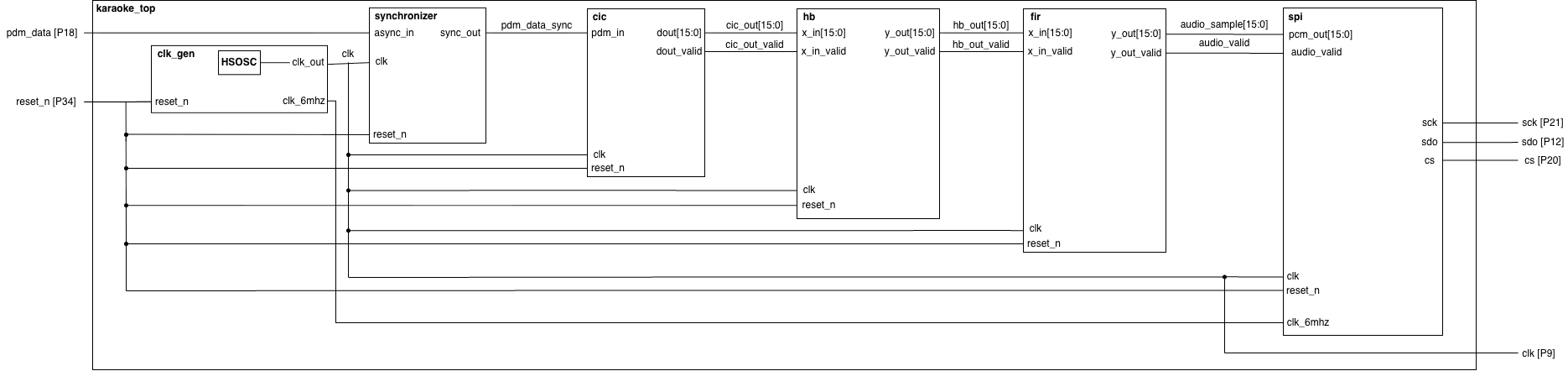
The block diagram in Figure 6 depicts the general architecture implied by the SystemVerilog code.

Our inputs are the reset on the dev board and the continuous single-bit stream of data, pdm_in, from the microphone. The clk_gen module generates the internal 1.536 MHz clock and the 6 MHz clock that drives the 3 MHz SPI. The pdm_data input is first put into a synchronizer just in case since our leads are long (technically, the clk going out to the microphone should already have made sure of synchronization). The output data goes to the CIC (cic.sv), where it is transformed into a 16-bit, 64 kHz PCM with a validity signal that pulses whenever a new value is available. Those two signals then pass into the half-band filter (hb.sv), where it transforms into a 32 kHz PCM with a specific passband and stopband, along with some passband ripple and stopband attenuation. Then, these values are passed along to the final filter, the FIR (fir.sv), where it is finally decimated by another factor of 2 down to 16 kHz, and its ripple and stopband attenuation are corrected. The 16-bit values and the validity signal are finally passed into the SPI (spi.sv), where a sck, sdo, and cs signal are generated every 16 kHz on a 3 MHz SPI signal using cross-domain clocking. (TLDR: A new 16-bit PCM value is shifted out from the MSB to the LSB on the 3 MHz clock, with the FPGA acting as the master and the MCU as the slave.)

Schematic

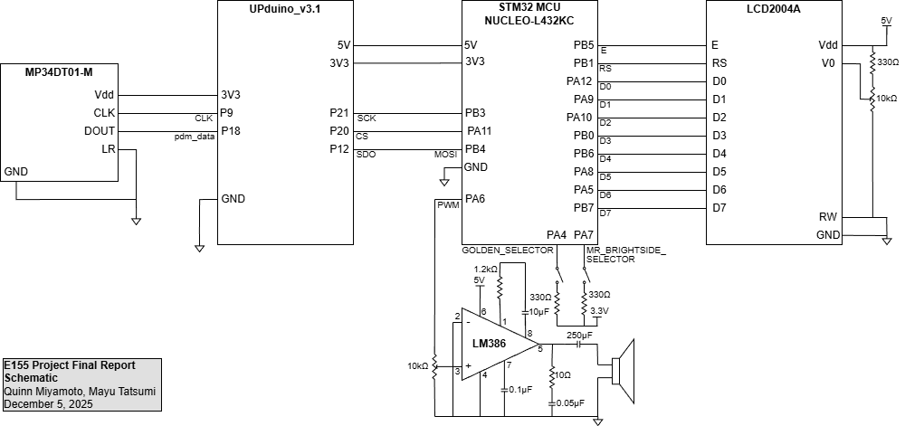
Figure 7 above depicts the physical connections between all of the project’s necessary electronic components. This includes the PDM microphone, LCD screen, speaker, audio amplifier, switches, FPGA, and MCU.

Note that the microphone and FPGA interfacing is done in accordance with the MP34DT01-M datasheet. The most prominent feature of note is the tying of the LR port to ground, as that configures a pdm_data signal pattern of valid data when the CLK signal is low and high impedance when CLK is high.

Additionally, the MCU has direct, one-to-one pin connections with the LCD, with the exceptions being RW and V0. RW is tied directly to ground because we are only performing Write operations with the LCD and never Read ones, so the bit never needs to be set; by just wiring it to ground instead of sending a zero to the pin every time, this allows us to free up MCU ports that we can use for other, more important connections. Meanwhile, V0 is wired to the output of a 10 kΩ potentiometer, so that the contrast between the backlight and the characters being displayed can be controlled.

Furthermore, the MCU-audio-amplifier-speaker circuit shown at the very bottom is yet another component taken from Lab 4, affording the users the ability to modify the speaker’s volume.

However, most notably of all, is the fact that MCU pins PA5 and PB7 are no longer connected, nor are PA6 and PB6. Previously, while it is not noted on the PCB schematic we are given for this class — or anywhere easily found in official STM32 documentation, for that matter — those two pairs of pins share respective connections via two surface-mounted 0 Ω resistors. This was rather frustrating to discover, as we were struggling with the LCD showing randomly inserted, completely incorrect characters for the longest time. As it turns out, because the LCD (without using I2C to communicate) depends entirely on the accuracy of analog signals, it was confused when it received voltages of 1.5 from those four pins, specifically — half of the 3.3 V signal it should have been getting. Seeing as 1.5 V is below the minimum threshold of 2.2 V to count as a high signal and above the maximum threshold of 0.6 V to count as a low signal, the LCD simply chose at random every time it encountered this problem. Thus, while difficult to portray in the above schematic, the removal of these resistors is perhaps the single-most important aspect of the circuit design to our team.

Flowchart

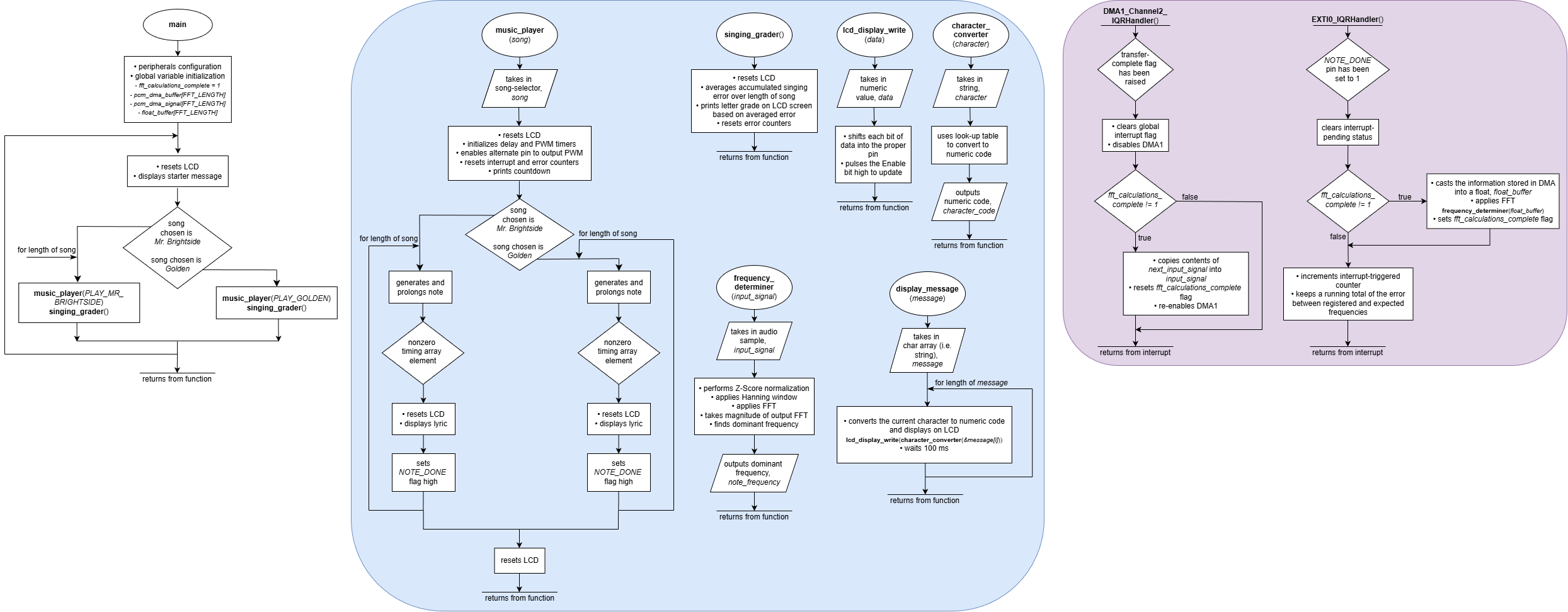
The Figure 8 flowchart provides a detailed overview of the microcontroller’s most significant routines. This is a visual depiction of the peripherals discussed in section MCU Design Overview above. In summary, there is a main loop that continuously polls for the user’s song selection; when a song is eventually chosen, the music_player() function outputs each note using PWM-generation and delay functions, interrupting after every note is done playing to FFT the user’s voice and subsequently determine their error. There is also an occasional interrupt that tells the program to output new lyrics on the LCD. Finally, the singing_grader() function informs the user of their error, before starting the process anew.

Results

Overall, our work on the project resulted in a resounding success! We achieved all of the goals we set out to meet, and had a wonderful time introducing others to our karaoke machine on Demo Day.

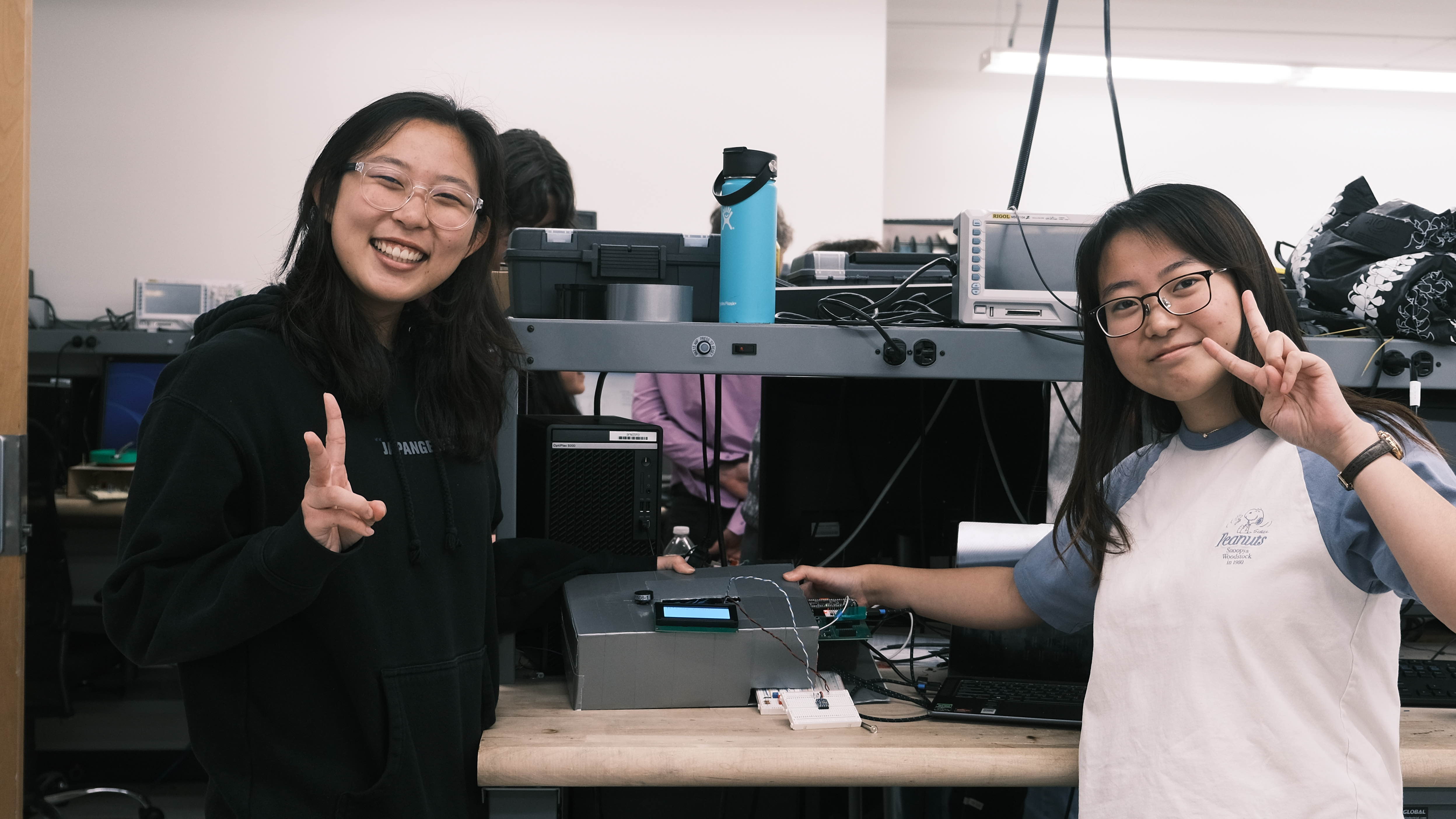
Evidence of our project’s functionality can be viewed in the following Figure 10, with the tester, Alan Kappler, attempting to sing Golden:

Figure 10: Demo video

Additionally, Figure 11 provides a close-up photo of our machine:

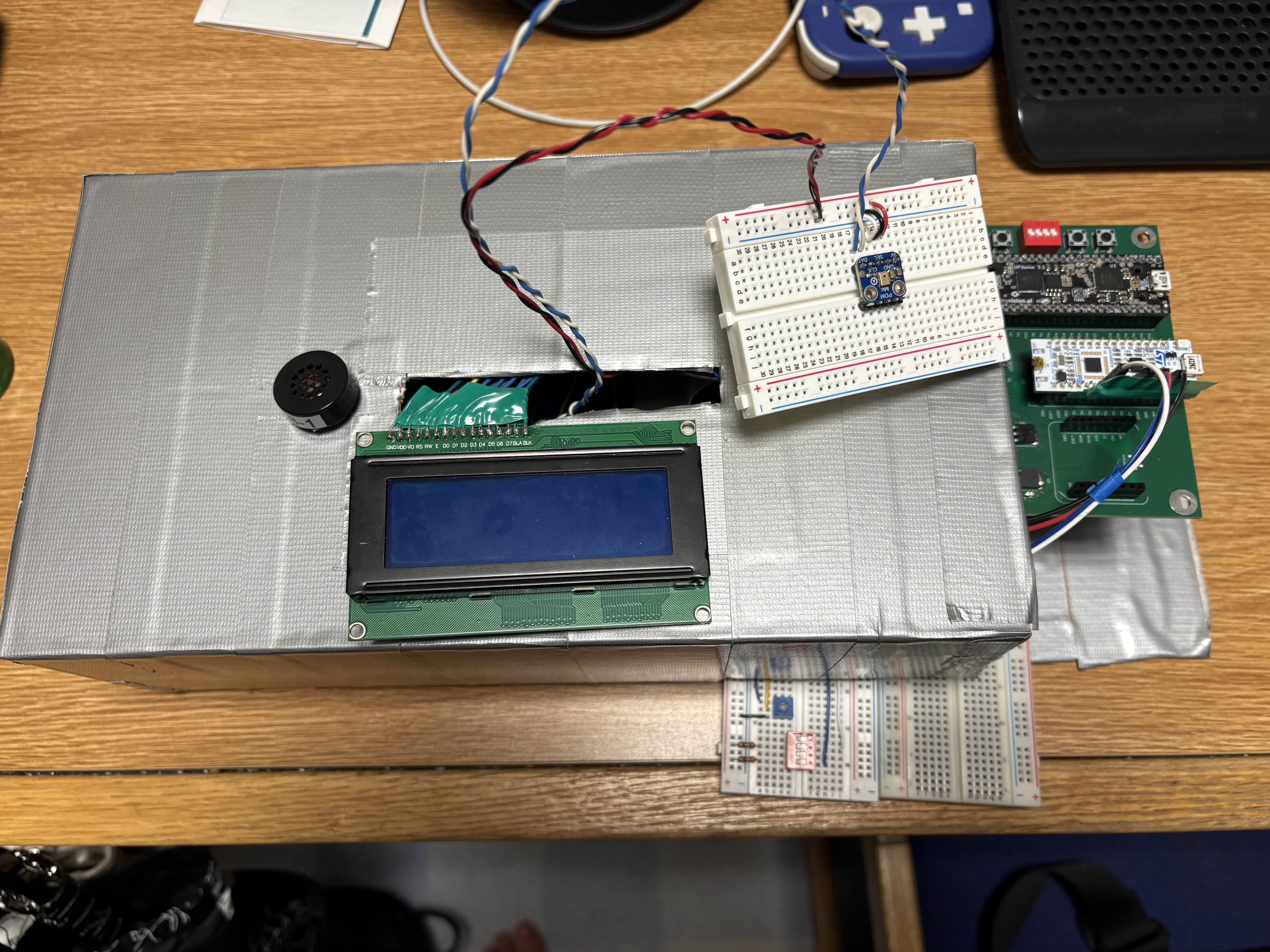
While it would have been nice to have a covering that isn’t just a cardboard box wrapped in silver duct tape, we are still rather pleased with our final product. As we are not mechanical engineers, it ultimately has a little charm to it :)

Specifications Status

Referring back to the specifications outlined above, we can more quantitatively define our success as follows:

Design allows the user to choose a song through external hardware → STATUS: Met!

The red switch on the breadboard allows for choosing between Mr. Brightside (switch 4) and Golden (switch 2) after boot, and the LCD screen displays the instructions / options if no song is selected.

Design detects input frequencies between 300 to 2000 Hz → STATUS: Met!

The microphone is able to detect frequencies between 250 Hz to 2400 Hz with a resolution of around 25 Hz. There is some latency when displaying detected frequencies on the LCD, mostly as a result of the LCD’s ability to refresh its display. It is much faster when printing in SEGGER in debug mode, though that is also bottle-necked by the printf function. For a higher resolution, a higher FFT length could be used, though it would result in a higher latency as well. The testbenches for the filters used to make this possible is displayed in the Testbenches section below.

Design scores the user’s singing by comparing detected and expected notes → STATUS: Met!

The design outputs a final score after averaging the amount of percent error based on each note expected. This is achieved by accumulating the percent error of each note and dividing the total at the end by the number of samples taken. We have implemented a lenient grading system as a result of the generally loud ambient noise in the Digital Lab and accounting for the talking during Demo Day, as found in this file.

Design plays back the expected song through a speaker as reference → STATUS: Met!
Design utilizes a pitch and delay media format (as seen in Lab 4) → STATUS: Met!

Regarding both specs: As stated earlier, we had to transcribe both songs, Golden and Mr. Brightside, into the Lab 4 {frequency (Hz), duration (ms)} format. The PWM and delay-timer code were similar to the lab code as well.

Displays properly-timed lyrics on an LCD screen → STATUS: Met!

As mentioned before, we wrote our own display_message() function for the LCD, which we are now able to pass lyrics through in order to display the desired words on the screen. This is supplemented with the timing matrix, which syncs up the lyrics change with the exact beat we want. The evidence of this success can be viewed in the demo video above.

LCD display does not flicker → STATUS: Met!

Again, evidence of this success can be viewed in the demo video above.

Testbench Simulation

Seeing as software verification is just as important as hardware verification — as well as extremely useful when it comes to debugging — we have created various testbenches to aid us in rigorously proving that our filters, in particular, work.

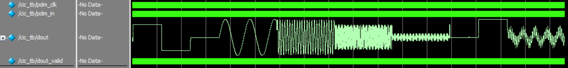
First and foremost, we have the Figure 12 waveform outputs of our CIC filter. Here, a PDM input with various 1/0 densities represents a +1, -1, 0, sin(500), sin(5000), sin(15000), and sin(30000), along with an impulse, a step response, and a mixed signal of a combined 1000, 8000, and 25000 Hz. You can see that the 1-bit signal is converted into a 16-bit, 64 kHz signal with the 15 kHz and 30 kHz attenuated out, as expected.

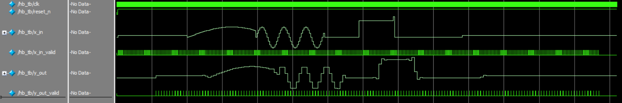
Next, we have our half-band filter in Figure 13. You can see that the validity signal, passed in at 64 kHz, is decimated by 2 down to 32 kHz (compare x_in_valid and y_out_valid). You can also see the same in the signals that are passed through, along with some latency.

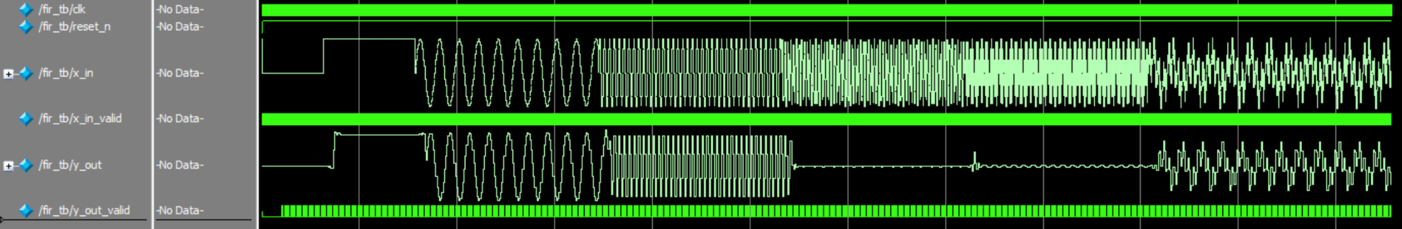
Again, with our Figure 14 FIR testbench output, you can see that the validity signal gets decimated by 2 down to 16 kHz and that the output signal gets choppier as a result. Also, some attenuation occurs at frequencies of 7 kHz and 14 kHz, which is as expected.

Finally, with the Figure 15 image, we can see evidence of our SPI transaction’s success. We passed in values through pcm_out, and you can see the correct values being passed through SCK (though only 0x0000, 0xFFFF are easy to read). The SPI runs at 3 MHz, but realistically, after the three filters, expected outputs come out at a frequency of 16 KHz, which is the width between inputs of 0x1234, 0x5678, and 0x9abc (so you would see this speed on the logic analyzer being fed into the MCU).

Oscilloscope Traces

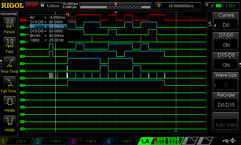
Last but not least, we used a Logic Analyzer in Figure 16 to aid us in proving that the LCD works as expected. Here, we tried to write the message “uPs!” on-screen, which corresponds to binary codes of “01110101,” “01010000,” “01110011,” and “00100001,” respectively (with the most significant bit being what is passed in to D7 and the least significant bit being passed into D0). Evidently, we can see that after RS goes high for the first time (which is actually signified on D9 in the above image), the traces match exactly what we expected.

References

E155: Course website.

STM32L432KC Datasheet: STM32 MCU datasheet.

STM32L432KC Reference Manual: STM32 MCU reference manual.

Quinn Miyamoto’s E155 Portfolio: Team member Quinn Miyamoto’s portfolio of this course’s labs.

Fix That Note! E155 Final Project Portfolio: Past E155 portfolio for the Fix That Note! project, which involved telling a user what note their system was detecting.

An Intuitive Look at Moving Average and CIC Filters: A series of blogs made by Tom Verbeure on designing a pipeline for audio decimation and filtering.

FIR Halfband Filter Design: A MATLAB guide to designing half-band filters, used in conjunction with the DSP-Related article below.

Simplest Calculation of Half-band Filter Coefficients: An online guide to designing half-band filter coefficients.

jaycordaro/half-band-filter: An implementation of a half-band FIR filter, from MATLAB to fixed point in SystemVerilog.

MEMS audio sensor omnidirectional digital microphone: Datasheet for MP34DT01-M.

Interface 16×2 LCD with STM32 (No I2C) — 4-bit Guide: A guide to interfacing an LCD with an STM32 MCU with an 11-line parallel bus, instead of I2C.

STM32 LCD 16×2 Library & Example | LCD Display Interfacing: A guide to initializing and writing to an LCD using an STM32 MCU.

I2C Serial Interface 20x4 LCD Module: Datasheet for the LCD’s HD44780 controller chip.

MC21605A6W-FPTLW: Alternative LCD datasheet.

Generating signals with STM32L4 timer, DMA and DAC: A guide to interfacing DMA with SPI.

Fast Fourier Transform using the ARM CMSIS Library within the STM32 MCUs: A video tutorial on how to pick a dominant frequency out of a given signal on the STM32 MCU, using ARM math functions (including the FFT).

Normalizing Signals for Enhanced Analysis and Interpretation: A guide to normalizing signals as preparation for Fourier Transforms.

STMicroelectronics/cmsis-core: GitHub repository of all ARM math functions.

Acknowledgements

We would like to thank the entire MicroPs teaching team for their help in getting this project off of the ground this semester, especially Kavi Dey (’26) and Prof. Spencer. Additionally, special thanks goes out to Cole Plepel (’27) for transcribing our karaoke machine’s music. We really appreciate you!